Overview Graph Analysis
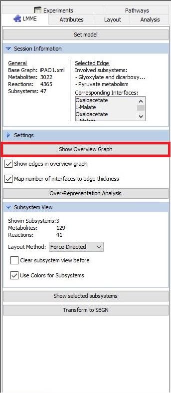
If you press the button Show Overview Graph, the decomposition method will be executed. From the resulting subsystems, a graph structure is determined by inserting one node per subsystem and an edge between two of these nodes whenever there is at least one interface metabolite between the two subsystems.
The resulting overview graph is then shown on the left side of the application window.
Layout
There are several available layout methods than can be used for the visualisation of the resulting overview graph. We will give a short description of them in the following.
- Force-directed Layout
At the moment, LMME uses the implementation of the Spring Embedder, that is available in Vanted. The main idea is to use a physical analogy to create a visually appealing drawing of a graph. Physical forces are assumed in two ways: attractive force between adjacent vertices and repulsive forces between any pair of vertices. Node movement according to these forces is then computed iteratively until a force equilibrium is reached. See the publication below for more details.
Eades, P. (1984). A heuristic for graph drawing. Congressus numerantium, 42, 149-160.
- Grid Layout
The vertices are placed on a grid (integer coordinates) to improve readability and reduce clutter.
- Circular Layout
All nodes are placed on a circle. A heuristic approach is applied to reduce edge crossings by changing the order of the nodes on the circle.
More layouts are available via the Layout tab provided by Vanted. In addition, we plan to extend the available layouts in the future.
General Analysis
As soon as the overview graph is shown, we have two possibilities to directly change its appearence.
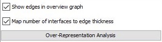
The Show edges in overview graph checkbox controls whether the edges in the overview graph are visible. If there are a lot of edges, but you are actually only interested in the individual subsystems itself instead of their relationships, this option may be what you are looking for.
The Map number of interfaces to edge thickness checkbox controls whether the number of interface metabolites that exist between two subsystems is represented by the thickness of the corresponding edge. The more interfaaces there are between two subsystems, the thicker the edge between those subsystems will be, if this checkbox has been ticked.
Over-Representation Analysis
An Over-representation analysis (ORA) can be used to find groups of metabolites that have an unexpectedly high proportion of metabolites of significantly low or high concentration. To run ORA, several preconditions need to be satisfied:
- You need measurement data of the concentration of several metabolites of the model
- You need a list of metabolites with significantly lower or higher concentrations (in the following we simply call them significant metabolites)
- You can have a list of reference metabolites ((e.g. the total set of metabolites that have been measured during an experiment). If not provided, the reference set will simply default to the set of all metabolites that are contained in the model.
- You need a decomposition of the metabolites into groups
If you now want to compare the proportions of significant metabolites between those groups, ORA might be a good choice.
If you click on the button Over-Representation Analysis, the ORA settings appear. You can choose two files to load there. The first is a list of significant metabolites, while the second is optional and expects the list of reference metabolites (e.g. the total set of metabolites that have been measured during an experiment). If not provided, as said before, the reference set will simply default to the set of all metabolites that are contained in the model.
The lists that you load should be normal plain text files, having only one column that contains the SBML IDs of the respective metabolites, one per row, as can be seen in the example below:
cpd01
cpd03
cpd08
First, the ratio between the number of significant metabolites and the number of reference metabolites is computed. If all subsystems behave the same, we would expect to have more or less the same ratio within all of the subsystems at hand. Using a Fishers exact test for every group of metabolites, it is tested whether the ratio within a group is significantly different from the overall ratio. In addition, the False Discovery Rate is used to correct for multiple testing.
If a subsystem turns out to be significant, its corresponding node in the overview graph is coloured red, while the other subsystems remain white.
For more information on the following, see the mentioned publications.
- ORA
Khatri, P., Sirota, M., & Butte, A. J. (2012). Ten years of pathway analysis: current approaches and outstanding challenges. PLoS computational biology, 8(2), e1002375. doi.org/10.1371/journal.pcbi.1002375
- FDS
Benjamini, Y. and Hochberg, Y. (1995), Controlling the False Discovery Rate: A Practical and Powerful Approach to Multiple Testing. Journal of the Royal Statistical Society: Series B (Methodological), 57: 289-300. doi:10.1111/j.2517-6161.1995.tb02031.x