Model Decomposition
Having loaded a model, we can now compute a decomposition. Currently, LMME supports four decomposition methods:
- Predefined Decomposition
- KEGG Decomposition
- Compartment Decomposition
- Decomposition by Schuster et al. (2002)
The overall idea is to derive a set of subsystems, which formally are subgraphs of the graph that is associated with the model of interest. Having this set of subsystems, we look for metabolites that are exchanged between them (interface-metabolites). As interface metabolites represent relationships between subsystems, this leads to another graph structure - the overview graph - containing a node per subsystem and an edge between two subsystems if there are interface metabolites between these subsystems. Some of the subsystem nodes may then be chosen to create a detailed view of their relationships in form of a consolidated subsystem graph.
Please note that a subsystem always needs to reflect the contained reactions in a thermodynamically feasible way, meaning that any reaction contained in a subsystem always is connected to exactly the same metabolites as in the underlying model. A subsystem hence is already determined by its reactions. Thus, we sometimes only refer to the reactions of a subsystem, implicitly assuming that all of the involved metabolites are also part of the subsystem.
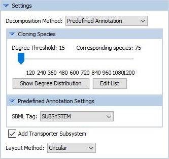
The figure shows the related part of the settings, which we will now discuss in detail. In the drop-down menu Decomposition Method, we select one of the methods. Having done that, the Cloning Species settings may appear or disappear, depending on whether the selected method expects cloning or not. The meaning of cloning is going to be described below. In addition, there will be a specific settings part where we can specify the settings for the selected method. This will also be described below as part of the descriptions of the individual decomposition methods.
More information on the available layouts can be found on the subpage Overview Graph Analysis.
Cloning
On the network level, cloning means to replace a node, that may have several neighbors, by several individual copies of itself, each having an edge to exactly one of the former neighbours of the replaced node. This on the one hand improves readability of the network and on the other hand avoids the detection of meaningless interfaces between subsystems in further stages of the procedure. As one can imagine, two systems that may both involve a common metabolite like ATP, do not necessarily have a meaningful relationship with one another.
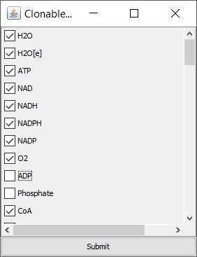
The settings part for the cloning has a slider for the Degree Threshold. This represents the minimum degree (minimum number of reactions, a metabolite is involved in), such that metabolites having at least the specified degree are going to be cloned. However, clicking the button Edit List allows us to edit the list of metabolites that are going to be cloned, as the degree itself may not always be the best way to detect this kinds of metabolites. Within the appearing window (see figure), we can simply untick those metabolites that we do not want to be cloned and tick those, that we want to be cloned although they might not meet the degree criterion.
When changing the value of the slider, there will be an immediate update of the number of corresponding species having this degree.
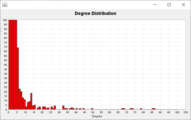
In addition, we can have a frequency distribution plot (see figure) of the occuring degrees throughout the network shown when clicking the button Show Degree Distribution. This is meant to assist us in finding a reasonable degree threshold for the current model.
We will now give an overview of the currently implemented decomposition methods.
Predefined Decomposition
This method is based on an existing decomposition of the model, which is contained in the underlying SBML file of the model in the form of reaction notes. Reactions in this case are required to have assigned the name of the subsystem that they belong to.
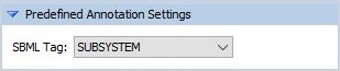
In the corresponding setting (see figure), there is a drop-down menu, containing all note names that have been found in the file. Currently, LMME is able to read notes of the same form like SUBSYSTEM and KEGG shown in the following minimal example:
<reaction>
    <notes>
        <optionalLayer(s)>
            <p>
                SUBSYSTEM: Glycolysis
            </p>
            <p>
                KEGG: R00006, R00226
            </p>
        </optionalLayer(s)>
    </notes>
    ...
</reaction>
Note that the <optionalLayer(s)>-tags in this case literally represent optional layers that can but do not need to be present.
The only requirement is that there is a <p>-tag somewhere nested inside the <note>-tag, which is of the form
<p> [NoteName] : [NoteValue] </p>
In this case, [NoteName] is the term that you select in the settings drop-down menu and [NoteValue] contains the names of the individual subsystems that exist in this particular predefined decomposition.
KEGG Decomposition
This method uses the KEGG IDs, that have been assigned to the reactions, uses the information from KEGG, which reactions belong to which pathways, to finally determine a set of KEGG pathways that are very likely to be present in the model at hand.
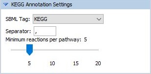
In the corresponding setting (see figure), there is a drop-down menu, containing all note names that have been found in the file, as well as the possibility to enter a separator in a textfield. The separator is used if there are more than one KEGG IDs assigned to a reaction. Currently, LMME is able to read notes of the same form like SUBSYSTEM and KEGG shown in the following minimal example:
<reaction>
    <notes>
        <optionalLayer(s)>
            <p>
                SUBSYSTEM: Glycolysis
            </p>
            <p>
                KEGG: R00006, R00226
            </p>
        </optionalLayer(s)>
    </notes>
    ...
</reaction>
Note that the <optionalLayer(s)>-tags in this case literally represent optional layers that can but do not need to be present.
The only requirement is that there is a <p>-tag somewhere nested inside the <note>-tag, which is of the form
<p> [NoteName] : [NoteValue] </p>
In this case, [NoteName] is the term that you select in the settings drop-down menu and [NoteValue] contains the names of the individual subsystems that exist in this particular predefined decomposition.
In addition, the settings for this decomposition contain a slider for the minimum reactions per pathway. This is part of the heuristic approach that is currently implemented and will be described below. For the moment, let's call this threshold t.
The following description is based on the one given in our [paper].
Let W denote the set of all reactions that provided a KEGG ID (W for working set). For any reaction R of W, the KEGG API is queried to find a set CR of candidate pathways that R might belong to. Having done this for all reactions in the working set W, the following heuristic approach is used to assign each R of W to a single final subsystem. We iteratively repeat the following steps until W is empty:
- For the KEGG pathway P that currently is contained in CR for the most reactions R of W, create a new subsystem SP.
- For any reaction R of W having P in CR, add R to the new subsystem SP and remove R from W.
- For any KEGG pathway P that is now contained in CR for less than t reactions R of W, remove P from CR. If CR is now empty, also remove R from W.
The reason for the usage of the threshold t is that it might occur that a particular KEGG pathway only occurs as candidate pathway for a few of the reactions by chance but is actually not part of the model at hand. Using this threshold directly prevents us from taking these pathways. The default value for t is 5 but you may change it depending on the model at hand.
Please note that, as every request to the KEGG API takes some time, the entire decomposition procedure may take a while. Therefore, at the bottom of the application window, there is a status message, informing you about the current proportion of processed reactions.
Compartment Decomposition
This method determines a decomposition of the model based on the compartment information available in the model.
Metabolites are required to have a compartment affiliation in their <species>-tag inside the underlying SBML file, like it is shown in the following example.
<species id="c2" name="ATP" compartment="c">
First, the compartment information is read for each of the metabolites.
Second, every reaction is classified as either lying in one of the compartments itself or as being a transport reaction. If all metabolites that are involved in the reaction (reactants as well as products) belong to the same compartment, the reaction is also assigned to this compartment. Otherwise, it is considered a transport reaction.
Finally, this results in a decomposition containing one subsystem per compartment and the transporter subsystem.
Decomposition by Schuster et al. (2002)
This method is an implementation of the method that has been proposed in the following paper:
S. Schuster, T. Pfeiffer, F. Moldenhauer, I. Koch, T. Dandekar, Exploring the pathway structure of metabolism: decomposition into subnetworks and application to Mycoplasma pneumoniae, Bioinformatics, Volume 18, Issue 2, February 2002, Pages 351–361, https://doi.org/10.1093/bioinformatics/18.2.351
In contrast to some of the previously mentioned decomposition methods, this method does not rely on additional information contained in the SBML file but computes a decomposition solely from the network strucutre of the model at hand.
The idea is to temporarily remove metabolites that have a degree greater or equal to a specified threshold and consider the resulting connected components of the graph as subsystems.
However, as we would like to end up with an overview graph that contains meaningful relationships between individual subsystems, we decided to include the cloning procedure and slightly extended the approach in the following way.
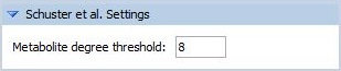
You as a user specify one degree threshold for the cloning as well as one for the decomposition itself. As the cloning will be performed first, the cloning threshold needs to be greater than the one for the decomposition itself. This now has the effect that we make use of the benefits discussed in the cloning section, while all of the metabolites having an initial degree between the two thresholds are used for the decomposition procedure and can be considered interfaces.
The current defaults are 15 for the cloning threshold and 8 for the decompsition threshold, which we found during testing the tool with several models. Feel free to explore them further.
Transporter Subsystem
In the settings panel, there is a checkbox labeled with Add Transporter Subsystem. If you check it, there will be one additional subsystem in the resulting decomposition which contains all transport reactions. Please note that, independent of the chosen decomposition method, the transport reactions will all be put in the transporter subsystem.
Default Subsystem
It may sometimes occur, that there remain unclassified reactions after a decomposition has been performed (e.g. as it may be the case that not all of the reactions provided a KEGG ID when running a KEGG Decomposition). In this case, all of these reactions are added to the so-called default subsystem.